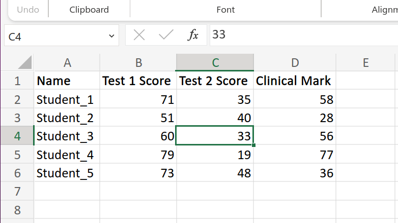
A basic introduction to spreadsheets

Warning: This is an extremely basic introduction to spreadsheets and may bore you. If you are comfortable entering data into a spreadsheet, this is most certainly not for you...but read on if you like.

I cover spreadsheet layout, formulas, conditional formatting and sorting an filtering. Other topics will be covered in later posts.

Can I use software other than Excel?

First things first...does it have to be this software? Can I use Microsoft Excel alternatives such as LibreOffice Calc and Google Sheets? The answer is a resounding yes! So what's the difference? Well, on the surface, and for the average user, it's probably just the same, but for more advanced users there may be significant differences. The respective user interfaces are also different, so it may be better to go with what you already know.

To many, the biggest difference may come down to one single factor - price. At the moment both LibreOffice Calc and Google Sheets are free to use...but Excel is not. Depending on your specific needs, this extra fee may be worthwhile as Microsoft Excel is most certainly the market leader when it comes to spreadsheets and is likely the most feature-rich environment. However, many occasional users may not need all these features. For a visual explanation of the differences, consider watching this introductory video.

Layout

Task: Download the companion spreadsheet here


Regardless of the specific software used, there are certain fundamental aspects in common to all spreadsheets. One of these shared aspects is the grid of rectangles you are greeted by when you start the program (or web application as it may be). This grid is organised into rows and columns. Rows are assigned numbers as identifiers and columns are assigned letters of the alphabet. Rows proceed predictably from 1 to... well however many rows your software allows (north of one million for Excel at the time of writing, but this may change with time). Columns are labelled A through Z, then follows AA, AB, etc. There are significantly fewer columns allowed (around sixteen thousand if you use Excel, but I hope you don't get there in daily use). The intersection of a row and a column, that is one rectangle, is called a cell. I suppose the cell can be called the functional unit of a spreadsheet. A specific cell is named using the column letter(s) followed by the row number. Figure 1 demonstrates this below.


Figure 1: Screenshot from Excel's online platform with cell C4 selected


It is important to know how to address certain rows, columns, and cells as this will be useful once formulas are applied.

Sheets

In general you will be able to have multiple sheets in a single file. There are cases where you will not, but these exceptions fall outside of the scope of this introduction. Sheets can generally be seen at the very bottom left of the screen, usually with a default name of "Sheet1", "Sheet2", etc. The sheet tab is illustrated in figure 2.


Figure 2: Sheet selection in Google Sheets, Excel, and LibreOffice Calc (from top to bottom)


Adding a new sheet is as simple as clicking on the plus sign (+) to add a new sheet. Sheets can separate related data, making data easier to organise and interpret while still giving you the ability to link different sheets through formulas. Sheets can be renamed by double-clicking the sheet name.


Task: Look at the sheets available on the companion spreadsheet. Add a few and try to rename them.


Entering data

First you need to decide whether to organise your data by row or column. Using columns is probably the most popular method, but both methods, or some combination of these can be useful depending on the application. We'll mostly use columns in this document. Although entirely optional (especially in small, single use applications such as quickly calculating the cost of a certain item), it is customary to give a column or row a name. Figure 1 shows the assignment of headings "Name", "Test 1 Score", etc.

Data can be entered manually or pasted into place. I don't think it's worth elaborating on entry or pasting since these are basic concepts in day-to-day computing. However there are a few features of data entry that are worth elaborating on.

Formatting of text

Text can be formatted in different ways. The standard list of commands such as bold, italics, justification of text, etc. are available and easily located. There are functions to format numbers as currencies, times, dates, number of decimal places, etc. Keep this in mind as you look over spreadsheets.

I'll go over decimal places as this is probably the most useful of these. A range of numbers (which could be one or millions of numbers) is selected. Right click on this selection and you should see that a menu comes up. There will be an option to format text or numbers (the names may differ between). Select this and modify the format according to what you in the box that comes up. Figure 3 demonstrates changing the number of decimal places using Microsoft Excel's web platform. Other platforms or versions may be slightly different in their placement of these menus or their naming conventions, but they all generally have similar functionality.


Figure 3: Manipulation of the number of decimal places


Task: Change the number of decimal places in the "Average" column on the "Number Format" sheet of the companion spreadsheet.


There is actually an easier way to manipulate the number of decimal places in Excel. There are buttons on the ribbon that does exactly that. In figure 4 the buttons to reduce and increase the number of decimal places are shown (the ones with the arrows).


Figure 4: Shortcut to the manipulation of the number of decimal places


Dragging

Duplication of data is a useful function when using spreadsheets. This can be accomplished by the process of "dragging". This process is demonstrated visually in figure 5, but basically you fill your cell with some text, then, making sure the cell is selected, hover over the block at the bottom right of the cell, apparently called the "fill handle", until your cursor changes its form to a plus sign (+). Once this has happened you can hold down the left mouse button on the fill handle, pulling it down to the desired cell. This process works over rows and columns.


Figure 5: Duplication of data on LibreOffice Calc by dragging down over multiple rows


This process also becomes useful when entering formulae (which will be discussed later in this post). Another useful aspect of dragging is that data demonstrating an inherent sequence can be, let's call it "intelligently", identified. Dragging allows continuation of this sequence. There may be slight differences between the functionality of dragging in terms of continuing sequences. In a test I performed I found that LibreOffice Calc will often create this sequence with just one value, for instance dragging with an initial value of 1 will yield 1, 2, 3, 4, ..., etc. Both Google Sheets and Microsoft Excel require at least two values. Figure 6 demonstrates this process in Google Sheets where it works quite well until the (unreasonable) task of generating primes is expected.


Figure 6: Demonstration of series generation by dragging on Google Sheets


This may not necessarily work as expected in certain instances. One of these is the case of LibreOffice Calc, where you just want a series of 1s and it produces the series 1, 2, 3, 4, ... etc. This may often be remedied by placing more than one of the same value below each other and then selecting both and dragging. Another annoyance may come up when you want to repeat a sequence, let's say 1, 2, 1, 2, 1, 2... This will generally result in some arbitrary sequence the program generated based on some algorithm. Fortunately this happens little enough for most occasional users and the desired outcome can often be obtained as a result of copying and pasting a few times. More advanced techniques fall outside of the scope of this particular post and may be addressed later.

To conclude this section, dragging the fill handle is a good method for duplication and series generation. Unfortunately this process fails in certain instances and is a symptom of using the same tool for two different functions.


Task: Open the "Dragging" sheet of the companion spreadsheet and drag the fill handle on all existing columns to see the result. Do them in different orders and see what results.

Ranges

A range is a list of cells in a spreadsheet. This can be arranged in a single column, a single row, have multiple rows and columns or may be made up entirely unconnected cells. This range can be separated by commas or colons.

Ranges may either be typed out or selected by dragging with or without the use of either the shift or ctrl key. It is difficult to demonstrate ranges as a concept outside of formulas and functions, so we will get back to it in those sections.


Task: On any sheet select cells and ranges. Use the shift and ctrl keys as described. See if you can identify the ranges of continuous sections you select.

Formulas

A formula is just a procedure assigned to a certain cell which takes data in other cells, transforms it, and displays the result in the initial cell. This is extremely useful and is, at least to me, where spreadsheets do most of the heavy lifting in daily life.

To start a formula you need to select an empty cell and press the equal character (=) and then type the function required. The simplest way to use this is probably addition, subtraction, division, or multiplication of two numbers. In the case of adding two numbers we use the addition operator (+). To add the numbers 5 and 2 we simply enter = 5 + 2 into a cell and press enter. This will evaluate to 7. The same will apply to other arithmetic operations regardless of the number applied. Order of operations is respected, for instance = 1 + 2 * 3 evaluates to 7. This is demonstrated visually in figure 7.


Figure 7: Basic arithmetic in Microsoft Excel


These formulas are not necessarily confined to a single sheet. As your use of spreadsheets advances you may find a need to use formulas to link to different spreadsheets.

Now this is cool and all, but there is no difference between this and a basic calculator. More advanced techniques come into play with the use of functions.


Task: Create a new sheet and do some basic arithmetic as outlined in this section until you are satisfied you have the hang of it.


Structure of a function

A function has a few parts including:
  • Function name
  • Parentheses
  • Arguments

This structure is referred to as the syntax of the function. The function name is literally the word you type to use the function. This is placed immediately after the equals sign. Parentheses are placed right next to the function name and contain the arguments passed to the function (i.e., the arguments are placed inside of the parentheses). The information required to "make the function work" are the arguments. Arguments, depending on the function used, may be as simple as just the cells over which the formula is applied, or may require more information.

Functions therefore take the general form function_name(argument1, argument2, ...) after the equal sign. There is often a "tool tip" to guide the use of functions, but most can easily be searched online for clear instructions on their usage.

To demonstrate this concept, two basic functions will be used, SUM and AVERAGE.

The SUM function

The sum function is probably the easiest function to demonstrate: it simply adds all cells in a selected range. This is shown in figure 8.


Figure 8: Demonstration of the use of the SUM function


The sum function can work with more than one form of data. The first is a list of numbers which the user wants added. The second, more useful option is to define a range of values over which the summation must occur. The syntax for each is as follows:
List of numbers: =SUM(number1, number2, number3) where number1 etc. are just placeholders for actual numbers, for example, =SUM(1, 2, 3, 4, 5) which will yield an answer of 15 in the cell.

Summation over a range: =SUM(B2:B5) where B2 is the start of the range and B5 is the end of the range. This is literally just the same as adding cells B2, B3, B4 and B5. This would be meaningless with one argument (that is, adding just one number is not useful), but at its maximum the range it should be able to perform its function over is an entire row or an entire column. The range may also be over columns, rows, disconnected cells, or even some combination of this. Disconnected cells are separated by commas (e.g., =SUM(A2, B3, V3, Q3)).

You don't have to physically type in the cells or ranges if you don't want to. There is usually an option to click on individual cells. If multiple connected cells in rows, columns or a combination are required, this can be done by selecting the first cell in the range, then either holding the left mouse button down while dragging the selection to the last cell or alternatively selecting the first cell in the range, then, while holding down the shift key, selecting the last cell in the range. If individual disconnected cells are required this can be performed using the ctrl key.

The AVERAGE function

Often we need to find the average of a range of values. This may be useful in the case where we take multiple measurements or want an analysis of test scores of a class. The AVERAGE function is made for this purpose. The syntax for this function is: =AVERAGE(RANGE). This range works exactly as explained in the SUM function.

There is little more to explain regarding these functions. They are simple yet powerful and serves as the perfect entry into the world of functions. There are many more functions available, however they fall outside of the scope of this introduction.

Dragging formulas

We may want to copy formulas from one cell to the next. This is indeed possible and it will the program used will generally update the formula for use on the next row or column in a logical manner. For instance if in cell C1 I have the formula to add cells A1 and B1 (=SUM(A1, B1)), dragging downward from cell C1 to cell C2 will result in addition of cells A2 and B2 to with the result in cell C2 (i.e., =SUM(A2, B2)).

A word of caution: be sure to check at least a few of the cells you've dragged formulas into. There are cases where behaviour may be unexpected. These cases (and how to correct them) are outside of the scope of this introduction, but be warned that the convenience of using a spreadsheet with mathematical functions does not necessarily mean that you don't have to validate the outputs.


Task: On the "SUM & AVERAGE" sheet of the companion spreadsheet, use the SUM function to complete the first "Total" column for John. Drag the fill handle to complete all the other totals (Mary to Bill). After completion of the totals, use simple arithmetic in a formula to work out the percentage John received for the test. Once again, drag the fill handle to compute the percentages received by other students. Once that is done work out the averages for each question, the total and percentage using the AVERAGE function. Please do not type in numbers manually, but rather select the appropriate ranges when using functions and drag the fill handle as needed.


Weighted averages

The AVERAGE function above does not allow for the calculation of weighted averages. This is unfortunate as it is very often used, say for instance in a situation where two tests are written and they have different weightings. Fortunately though there are a few ways around this problem. A simple arithmetic way to obtain weighted averages in shown in Figure 9 where each component is multiplied by the weight.


Figure 9: Weighted vs unweighted averages


Task: On the "Number Format" sheet create a column called "Weighted Average" and calculate the weighted average of each student where test 1 counts 40% and test 2 counts 60%.

Conditional formatting

Conditional formatting is a way to assign a rule to a range of cells in order to change the appearance of individual cells in the selected range according to the value of the content of a the particular cell and often how it relates to other cells in the range. For instance some cells may be given different colours based on the value in the cell, perhaps the larger the value the lighter or darker it gets. This may be helpful to highlight the larger or smaller numbers in a range of cells, for instance showing who did well or poorly in a test.

You may assign certain rules or simply apply a colour scale to a range of values. Conditional formatting is an easy way to visually highlight certain aspects of data under study. Applying such formatting starts with selection of a range of cells to which the formatting should be applied. Application of a colour scale is demonstrated in figure 10.


Figure 10: Application of a colour scale to averages highlighting students who performed both well and poorly


Conditional formatting has many uses and the purpose here is just to demonstrate its application. This topic will be dealth with in greater depth in a later post.


Task: Apply a colour scale to the results on the "SUM & AVERAGE" sheet.

Filtering and sorting

Very often we have a lot of data and we want to filter or sort it according to certain values. To do this we simply select the column headings we wish to filter and sort across. In Microsoft Excel (and similarly for other packages) we simply click the "Sort & Filter" button and select the "Filter" option (with the funnel next to it). We now create little tabs next to each heading which allows us to filter by column. This is demonstrated in figure 11.


Figure 11: Demonstration of sorting and filtering in Microsoft Excel


A word of warning: I urge you to be careful when selecting these columns as unselected columns won't be sorted with selected columns...and this can be disastrous. Imagine a course where you want to admit top academic performers, but you only sort the results column. What you will find is that your name column will remain unsorted and it will now appear that students who are in reality not top achievers are given a spot in your course!


Task: Sort and filter the columns on the "SUM & AVERAGE" sheet and analyse the data as you like.


What was left out

There are many things that I left out in this post. One notable topic is charts and other graphics. These topics should be addressed in another post as their intricacies do not lend themselves to a superficial introduction. As I find time in my busy schedule I will definitely try to post more. Until then, try to cement these basic skills and explore the different options in the different menus you find in Microsoft Excel, Google Sheets, LibreOffice Calc, or whatever application you find yourself using.